NYC Parking Violations:
Scalable ETL &
Analytics System

Overview

New York City issues millions of parking violations each year. The data is publicly available but at over 20GB, it's not something you can simply download and explore. Raw records contain cryptic violation codes, inconsistent date formats, and no enrichment layer connecting a numeric code to what the driver actually did wrong.

This project built an end-to-end retrieval system to make that data usable: a pipeline that ingests from the NYC Open Data API, transforms and enriches it with PySpark, stores it in MongoDB, and serves it through an interactive Streamlit dashboard. The target user isn't a data engineer it's a city planner or policy analyst who needs to move from a question to an answer without writing a single line of code.

That framing shaped every design decision: what to clean, what to store, how to index, and what the dashboard surfaces by default. A system is only as useful as it is accessible to the people it's meant to serve.

Dashboard Demo

A live walkthrough of the Streamlit dashboard filtering by borough, month, and violation type to surface enforcement patterns across the city.

Business Problem

NYC's parking violation data is technically public but practically inaccessible at scale. The full dataset exceeds 20GB, making local processing impractical on most machines. Violation codes are numeric and meaningless without an external reference table. And without a structured query layer, answering even a simple question "which streets in Manhattan had the most violations last July?" requires hours of manual data wrangling.

The real problem wasn't storage or compute it was that no usable interface existed between the raw data and the people who needed to act on it. Municipal departments can't make evidence-based decisions about parking enforcement if getting to the evidence requires a data engineering project every time. This system was designed to close that gap permanently, not just answer one question once.

We also had to make a practical sampling decision: the full 20GB dataset exceeded local device limits, so we extracted a representative 1.1GB subset covering fiscal year 2023–2024. Key fields issue date, violation code, street code, vehicle type, and fine amount were spot-checked against the full population to validate that temporal and geographic patterns held in the subset.

ETL Pipeline

The pipeline follows four stages, each chosen for a specific reason rather than default tool selection.

One deliberate design choice: rather than imposing a rigid relational schema, we mirrored the API's output structure in MongoDB and layered aggregation at query time. This made the pipeline faster to iterate on and easier to extend to new fiscal years without schema migrations. The tradeoff slightly higher query complexity was acceptable given the read-heavy access pattern of the dashboard.

Stage 1 Extract: Paginated API Ingestion

The NYC Open Data API caps responses at 50,000 rows per request. A pagination loop accumulates up to 6 million records in batches, trimming to the exact target if it overshoots.

# Paginate NYC Open Data API to fetch up to 6M records
import requests, pandas as pd

target_rows = 6_000_000
limit = 50_000
offset = 0

url = f"https://data.cityofnewyork.us/resource/pvqr-7yc4.json?$limit={limit}&$offset={offset}"
violations_df = pd.DataFrame(requests.get(url).json())
offset += limit

while len(violations_df) < target_rows:
    next_url = f"https://data.cityofnewyork.us/resource/pvqr-7yc4.json?$limit={limit}&$offset={offset}"
    data = requests.get(next_url).json()
    if not data:
        break
    violations_df = pd.concat([violations_df, pd.DataFrame(data)], ignore_index=True)
    offset += limit

# Trim to exactly target_rows if we overshoot
violations_df = violations_df.iloc[:target_rows]
# → 6,000,000 rows fetched

Stage 2 Transform: PySpark Cleaning & Enrichment

PySpark handles date parsing, county code mapping, null treatment, and the join against an external violation code reference table turning numeric codes into human-readable descriptions and assigning the correct fine amount by borough.

from pyspark.sql.functions import col, to_date, year, month, upper, when, create_map, lit
from itertools import chain

# --- Clean & standardize ---
violations_spark_df = violations_spark_df \
    .withColumn("issue_date", to_date(col("issue_date"), "yyyy-MM-dd'T'HH:mm:ss.SSS")) \
    .withColumn("year",  year(col("issue_date"))) \
    .withColumn("month", month(col("issue_date"))) \
    .withColumn("street_name", upper(col("street_name"))) \
    .withColumn("violation_code", col("violation_code").cast("string"))

# Map county codes → readable borough names
county_map = create_map([lit(x) for x in chain(*{
    "NY": "Manhattan", "K": "Brooklyn", "Q": "Queens",
    "BX": "Bronx",    "R": "Staten Island"
}.items())])
violations_spark_df = violations_spark_df \
    .withColumn("county_name", county_map[col("violation_county")])

# --- Enrich: join violation code reference table ---
# Gives every record a plain-English description + fine amount
joined_df = violations_spark_df.join(violation_codes_spark_df, on="violation_code", how="left")

# Fine amount differs by borough; assign correct value per row
joined_df = joined_df.withColumn(
    "fine_amount",
    when(col("county_name") == "Manhattan", col("fine_amount_manhattan"))
    .otherwise(col("fine_amount_other"))
).drop("fine_amount_manhattan", "fine_amount_other", "violation_county")

Stage 3 Load: Write to MongoDB

The cleaned, enriched DataFrame is written to MongoDB via the Spark–Mongo connector. Pre-aggregated collections for each chart type are written separately so the dashboard queries pre-computed results rather than scanning the full collection at runtime.

# Write final dataset to MongoDB
final_df.write \
    .format("mongo") \
    .mode("overwrite") \
    .option("database", "nyc_parking_violations") \
    .option("collection", "parking_tickets") \
    .save()

# Pre-aggregate violation counts by type for faster dashboard queries
violation_type_agg = final_df \
    .filter((col("year") == 2023) | (col("year") == 2024)) \
    .groupBy("violation_code", "violation_description") \
    .count() \
    .toPandas()

spark.createDataFrame(violation_type_agg).write \
    .format("mongo") \
    .mode("overwrite") \
    .option("database", "nyc_parking_violations") \
    .option("collection", "violation_types_2024") \
    .save()

Stage 4 Visualize: Streamlit Dashboard

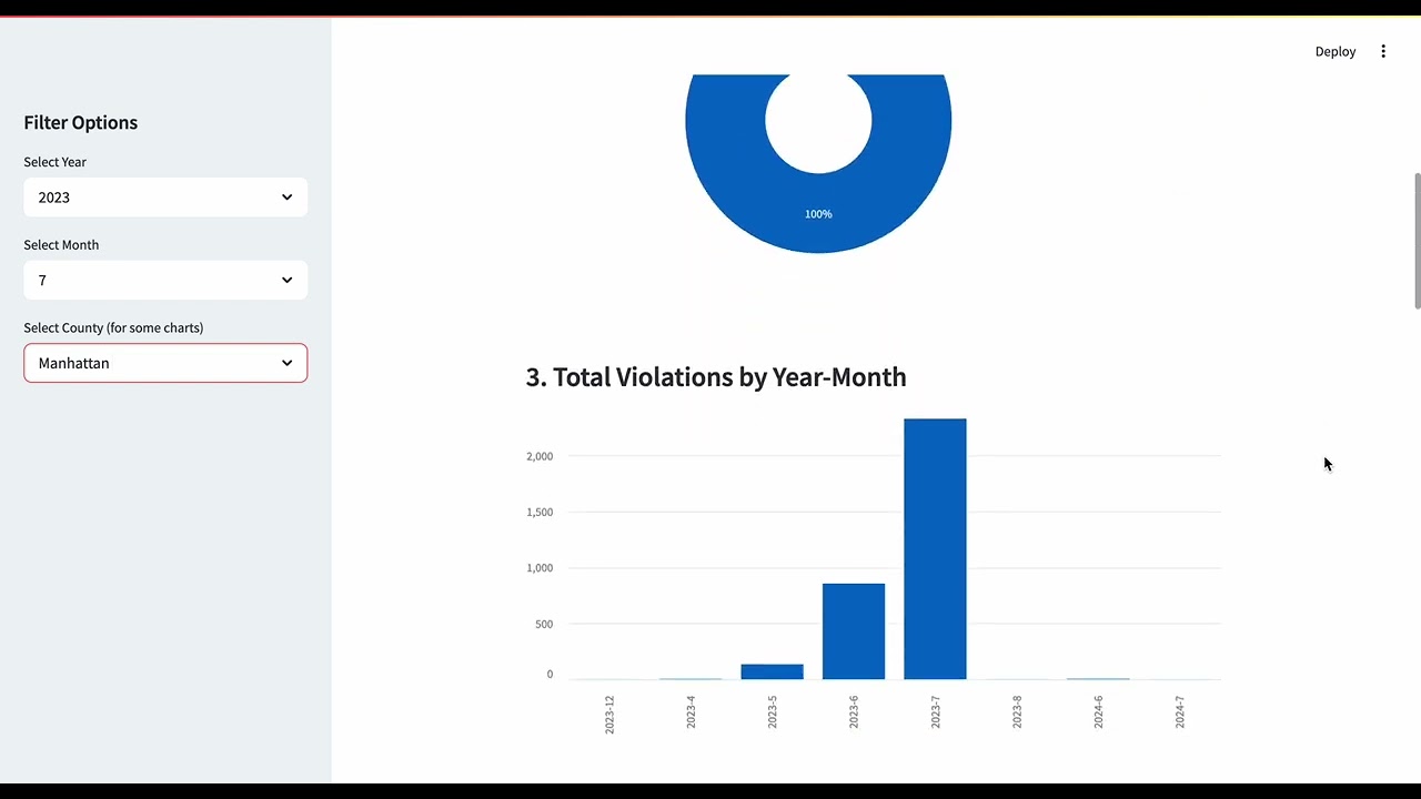
The dashboard reads from MongoDB and re-filters in memory. Sidebar controls for year, month, and county drive all seven charts simultaneously without page reloads.

import pandas as pd
import streamlit as st

df = pd.read_csv("finalpark.csv")
df["issue_date"] = pd.to_datetime(df["issue_date"], errors="coerce")
df["year"]  = df["issue_date"].dt.year
df["month"] = df["issue_date"].dt.month
df = df[df["year"].isin([2023, 2024])]

# Sidebar filters
selected_year   = st.sidebar.selectbox("Year",   sorted(df["year"].unique()))
selected_month  = st.sidebar.selectbox("Month",  sorted(df["month"].unique()))
selected_county = st.sidebar.selectbox("County", ["All"] + sorted(df["county_name"].dropna().unique()))

filtered = df[(df["year"] == selected_year) & (df["month"] == selected_month)]
if selected_county != "All":
    filtered = filtered[filtered["county_name"] == selected_county]

st.title("🚓 NYC Parking Violations Dashboard (2023–2024)")

# Chart 1 violations by type
st.markdown("### Violations by Type")
st.bar_chart(filtered["violation_description"].value_counts().head(10))

# Chart 2 borough distribution
st.markdown("### Borough Distribution")
county_dist = filtered["county_name"].value_counts()
st.plotly_chart({"data": [{"labels": county_dist.index, "values": county_dist.values,
                             "type": "pie", "hole": 0.4}]})

Key Insights

The system was validated through exploratory testing across different time and borough slices. Several consistent patterns emerged that would be difficult to surface from raw data alone.

Takeaways